Autoencoders

1. Introduction

Autoencoders are a specific type of feedforward neural networks where the input is the same as the output. They compress the input into a lower-dimensional code and then reconstruct the output from this representation. The code is a compact “summary” or “compression” of the input, also called the latent-space representation.

An autoencoder consists of 3 components:

1. Encoder
2. Code 
3. Decoder. 

The encoder compresses the input and produces the code, the decoder then reconstructs the input only using this code.

To build an autoencoder we need 3 things: an encoding method, decoding method, and a loss function to compare the output with the target.

Autoencoders are mainly a dimensionality reduction (or compression) algorithm with a couple of important properties:

• Data-specific: Autoencoders are only able to meaningfully compress data similar to what they have been trained on. Since they learn features specific for the given training data, they are different than a standard data compression algorithm like gzip. So we can’t expect an autoencoder trained on handwritten digits to compress landscape photos.
• Lossy: The output of the autoencoder will not be exactly the same as the input, it will be a close but degraded representation. If you want lossless compression they are not the way to go.
• Unsupervised: To train an autoencoder we don’t need to do anything fancy, just throw the raw input data at it. Autoencoders are considered an unsupervised learning technique since they don’t need explicit labels to train on. But to be more precise they are self-supervised because they generate their own labels from the training data

2. Architecture

Both the encoder and decoder are fully-connected feedforward neural networks. Code is a single layer of an ANN with the dimensionality of our choice. The number of nodes in the code layer (code size) is a hyperparameter that we set before training the autoencoder.

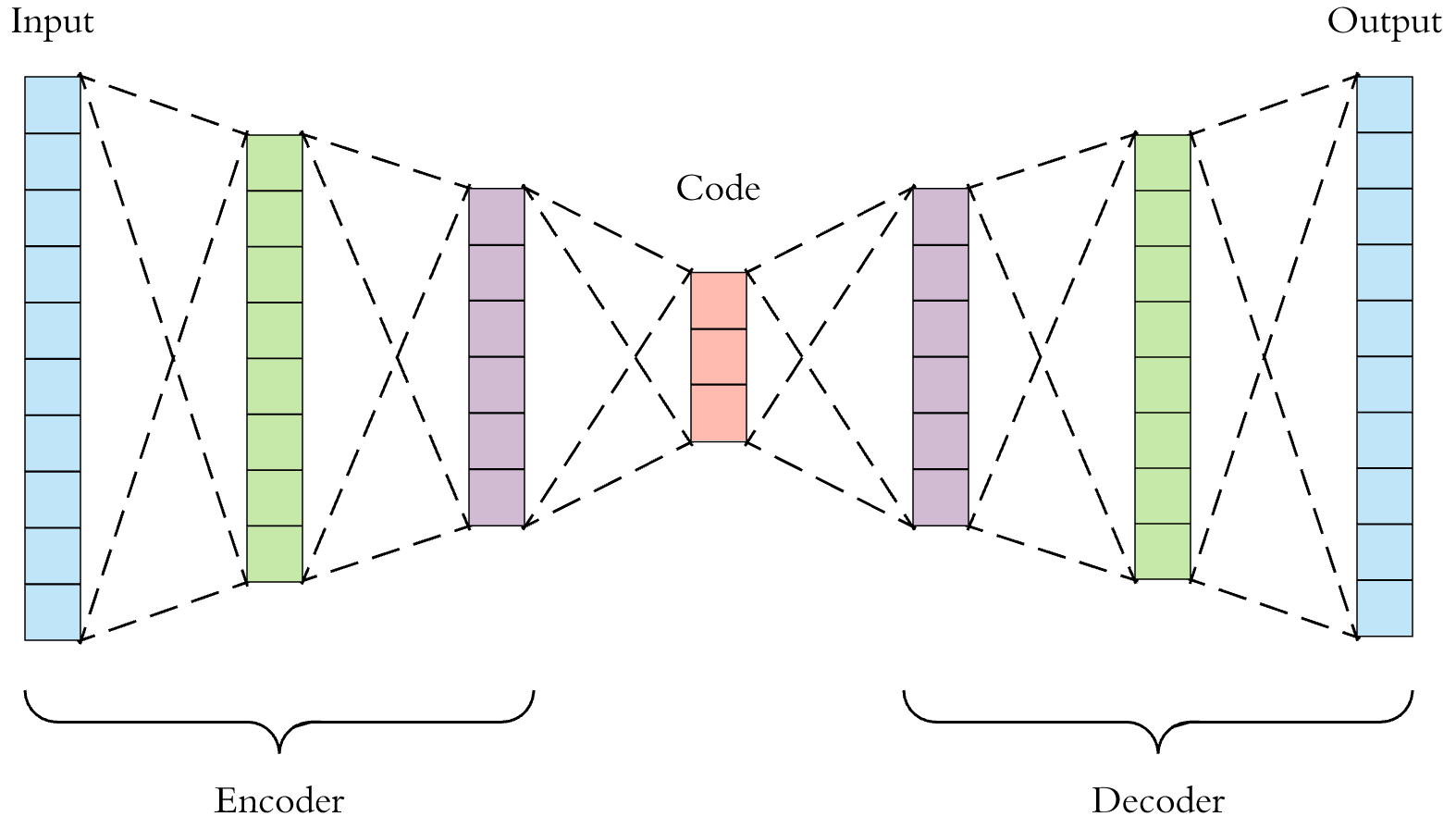
This is a more detailed visualization of an autoencoder. 

• First the input passes through the encoder, which is a fully-connected ANN, to produce the code. 
• The decoder, which has the similar ANN structure, then produces the output only using the code. 
• The goal is to get an output identical with the input. 
• Note that the decoder architecture is the mirror image of the encoder. This is not a requirement but it’s typically the case. The only requirement is the dimensionality of the input and output needs to be the same. Anything in the middle can be played with.

There are 4 hyperparameters that we need to set before training an autoencoder:

• Code size: number of nodes in the middle layer. Smaller size results in more compression.
• Number of layers: the autoencoder can be as deep as we like. In the figure above we have 2 layers in both the encoder and decoder, without considering the input and output.
• Number of nodes per layer: the autoencoder architecture we’re working on is called a stacked autoencoder since the layers are stacked one after another. Usually stacked autoencoders look like a “sandwitch”. The number of nodes per layer decreases with each subsequent layer of the encoder, and increases back in the decoder. Also the decoder is symmetric to the encoder in terms of layer structure. As noted above this is not necessary and we have total control over these parameters.
• Loss function: we either use mean squared error (mse) or binary crossentropy. If the input values are in the range [0, 1] then we typically use crossentropy, otherwise we use the mean squared error.

Autoencoders are trained the same way as ANNs via backpropagation.